International Summer School on Geospatial Data Science with R in Jena

We are proud to announce our “International Summer School on Geospatial Data Science with R” taking place at the GIScience department of Jena (Germany) from 25. August to 1. September 2019.

spat_logos

The summer school will consist of a mixture of lectures and lab classes and will teach advanced geospatial techniques for analyzing and predicting global change phenomena on the command line (mainly using R) in a fully reproducible workflow. This includes predictive modeling using statistical and machine learning techniques, model assessment and data science challenges with geospatial data. The summer school is generously funded by the German Academic Exchange Service which means that each accepted international participant will receive at least a funding of 450 Euros upon successful completion of the summer school.1 Application deadline is 15. May 2019.

Please share this fantastic opportunity with all interested parties and refer to the official website for more information on how to apply, the program and the invited lecturers.

We are looking forward to welcoming you in Jena!


  1. Applicants from Germany are welcome to apply but only a limited number can be admitted and no funding can be granted.

Geocomputation with R: workshop at eRum

geocompr_logo

This is a post by Robin Lovelace, Jakub Nowosad and Jannes Muenchow. Together we’re writing an open source book called Geocomputation with R. The project aims to introducing people to R’s rapidly evolving geographic data capabilities and provide a foundation for developing scripts, functions and applications for geographic data science. We recently presented some contents of the in-progress book at the eRum
conference, where Jannes ran a workshop on the topic. In this article we share teaching materials from eRum for the benefit of those who couldn’t be there in person and provide a ‘heads-up’ to the R-Spatial community about plans for the book. We’ll start with an overview of ‘geocomputation’ (and define what we mean by the term) and finish by describing how R can be used as a bridge to access dedicated GIS software.

Gecomp ‘base’ ics

The first thing many people will be asking is “what is geocomputation anyway”? As Jannes mentioned in his talk, the choice of name was influenced by the fact that the term seems to have originated in Leeds, where one of the authors (Robin) is based. The first conference on the subject was in Leeds in 1996, with associated extended abstracts including old-school computer graphics still available here; and there was a 21 year home-coming anniversary in 2017 where Robin and Jakub presented. A more practical reason is that the term is unambiguous: it’s about using computing techniques to do new things with geographic data, as indicated in Section 1.1 of the book. Our approach differs in one way from the early conception of geocomputation, however:

Unlike early works in the field all the work presented in this book is reproducible using code and example data supplied alongside the book (using R, a great language for reproducible research).

Like many open source projects R is evolving. Although ‘base R’ is conservative (as demonstrated in Roger Bivand’s keynote, in which he did a live demo using a version of R from 1997 that still runs!), the ‘ecosystem’ of packages that extend its capabilities changes fast (video here, slides at rsbivand/eRum18).

To clarify what we mean by ‘base R’, we can identify base packages with the following code (source: stackoverflow):

x = installed.packages()
row.names(x)[!is.na(x[ ,"Priority"])]

## [1] "base" "boot" "class" "cluster" "codetools"
## [6] "compiler" "datasets" "foreign" "graphics" "grDevices"
## [11] "grid" "KernSmooth" "lattice" "MASS" "Matrix"
## [16] "methods" "mgcv" "nlme" "nnet" "parallel"
## [21] "rpart" "spatial" "splines" "stats" "stats4"
## [26] "survival" "tcltk" "tools" "utils"

The output shows there are 28 packages that are currently part of the base distribution (R Core makes “base R” as Martin Maechler put it
during another keynote). These can be relied on to change very little in terms of their API, although bug fixes and performance improvements happen continuously.

The same cannot be said of contributed packages. Packages are created,
die (or are abandoned) and change, sometimes dramatically. And this applies as much (or more) to r-spatial as to any other part of R’s ecosystem, as can be seen by looking at any one of R’s task views. At the time of writing the Spatial task view alone listed 177 packages, many of them recently contributed and in-development.

In this context it helps to have an understanding of the history (Bivand, Pebesma, and Gómez-Rubio 2013). Like in politics, knowing the past can help navigate the future. More specifically, knowing which packages are mature or up-and-coming can help decide which one to use!

For this reason, after a slide on set-up (which is described in detail in chapter 2 of the book), the workshop spent a decent amount of time talking about the history of spatial data in R, as illustrated in slide 20. A more detailed account of the history of R-spatial is provided in section 1.5 of the book.

The slides outlining the basics of Geocomputation with R (which is roughly a synonym for r-spatial) can be found here.

Vector data

Spatial vector data are best used for objects that represent discrete borders such as bus stops (points), streets (lines) and houses (polygons). For instance, we can represent ‘Budapest’ (the city where eRum 2018 was held) as a spatial point with the help of the sf package (Pebesma 2018) as follows:

budapest_df = data.frame(
name = "Budapest",
x = 19.0,
y = 47.5
)
class(budapest_df)

## [1] "data.frame"

budapest_sf = sf::st_as_sf(budapest_df, coords = c("x", "y"))
class(budapest_sf)

## [1] "sf" "data.frame"

Why bother creating a new class if both objects contain the same essential data? It’s what you can do with an object that’s important. The reason for using the sf class can be understood as follows: it gives the budapest_sf spatial superpowers. We can, for example, now identify what country the point is using a spatial function such as a spatial join implemented in the function st_join()` (spatial subsetting would also do the trick, as covered in section 4.2.1). First, we need to load the ‘world’ dataset and set the ‘CRS’ of the object:

# set-up:
library(spData)
sf::st_crs(budapest_sf) = 4326

# spatial join:
sf::st_join(budapest_sf, world)

## Simple feature collection with 1 feature and 11 fields
## geometry type: POINT
## dimension: XY
## bbox: xmin: 19 ymin: 47.5 xmax: 19 ymax: 47.5
## epsg (SRID): 4326
## proj4string: +proj=longlat +datum=WGS84 +no_defs
## name iso_a2 name_long continent region_un subregion
## 1 Budapest HU Hungary Europe Europe Eastern Europe
## type area_km2 pop lifeExp gdpPercap geometry
## 1 Sovereign country 92476.46 9866468 75.87317 24016.3 POINT (19 47.5)

The slides describing vector data in R can be found here.
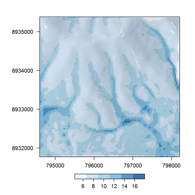
Raster data

On the other hand, a raster data represents continuous surfaces in form of a regular grid. You can think about a raster as a matrix object containing information about its spatial location. It has rows and columns, each cell has a value (it could be NA) and its spatial properties are described by the cell resolution (res), outer borders (bounding box – xmn, xmx, ymn, ymx), and coordinate reference system (crs). In R the raster package supports the spatial raster format (Hijmans 2017).

library(raster)
elev = raster(nrow = 6, ncol = 6,
vals = 1:36,
res = 0.5,
xmn = -1.5, xmx = 1.5,
ymn = -1.5, ymx = 1.5,
crs = "+proj=longlat")

The data structure makes raster processing much more efficient and faster than vector data processing.

elev2 = elev^2
elev3 = elev / elev2
elev4 = (elev2 - elev3) * log(elev)

elev_stack = stack(elev, elev2, elev3, elev4)
plot(elev_stack)

Raster objects can be subsetted (by index, coordinates, or other spatial objects), transformed using local, focal, zonal and global operations, and summarized. Importantly, there are many tools allowing for interactions between raster and vector data models, and transformation between them.

The slides associated with the raster data part of the workshop can be found here.

Visualizing spatial data

The spatial powers mentioned previously have numerous advantages. One of the most attractive is that geographic data in an appropriate class can be visualized on a map, the topic of Chapter 9 of the book. The workshop was an opportunity to expand on the contents of that chapter and ask: what’s the purpose of maps in the first place? To answer that question we used an early data visualization / infographic created by Alexander von Humboldt, illustrated below. The point of this is that it’s not always the accuracy of a map that’s most important (although that is important): the meaning that you wish to convey and the target audience should be central to the design of the map (in Humboldt’s case the unity of nature to an audience of Enlightenment book readers!):

In the context of geographic data in R, it is easier than ever to create attractive maps to tell a story. The previously created point representing Budapest, for example, can be visualized using the tmap package as follows:

library(tmap)
budapest_df = data.frame(name = "Budapest", x = 19, y = 47.5)
class(budapest_df)
#> [1] "data.frame"
budapest_sf = sf::st_as_sf(budapest_df, coords = c("x", "y"))
class(budapest_sf)
#> [1] "sf" "data.frame"
tmap_mode("view")
#> tmap mode set to interactive viewing
m = tm_shape(budapest_sf) + tm_dots() + tm_view(basemaps = "OpenStreetMap",
set.view = 9)
tmap_leaflet(m)

A range of mapping techniques were covered in the workshop including the plot() method from the sf package that generates multiple maps from a single object by default, such as this one representing the nz (short for New Zealand) object from the spData package:

More advanced maps were demonstrated, including this animated map of the United States (for information on how to make animated maps with R, see section 9.3) of Geocomputation with R.

The slides forming the basis of the visualization part of the tutorial can be found here.

Last but not least was a section on GIS bridges

Defining a Geographic Information System as a system for the analysis, manipulation and visualization of geographic data (Longley 2015), we can safely claim that R already has become a GIS. However, R has also its shortcomings when it comes to spatial data analysis. To name but a few, R is not particularly good at handling large geographic data, it is not a geodatabase and it is missing literally hundreds of geoalgorithms readily available in GIS software packages and spatial libraries. Fortunately, R has been designed from the beginning as an interactive interface to other languages and software packages (Chambers 2016). Hence, as long as we can access the functionality of GIS software from within R, we can easily overcome R’s spatial data analysis shortcomings. For instance, when attaching, the sf package to the global environment, it automatically links to GEOS, GDAL and proj.4, this means, the sf package gives the R user automatically access to the functionality of these spatial libraries. Equally, there are a number of packages that provides access to the geoalgorithms of major open source GIS Desktop software packages:

  1. rgrass7 provides access to GRASS7
  2. RSAGA provides access to SAGA GIS
  3. RQGIS provides access to QGIS. For much more details and background information, please check out the corresponding R Journal publication.

Note that you must have installed the GIS software on your machine before you can use it through R.[1]

In the workshop we shortly presented how to use RQGIS. The corresponding slides can be found here. In the book we additionally demonstrate how to use RSAGA and rgrass7 in Chapter 10.

Background on the book

Geocomputation with R is a collaborative project. We joined forces because each of us has been been teaching and contributing to R’s spatial ecosystem for years and we all had a similar vision of a book to disseminate R’s impressive geographic capabilities more widely.

As described in a previous article by Jakub, we’re making good progress towards finishing the book by the end of summer 2018, meaning Geocomputation with R will be published before the end of the year. The target audience is broad but we think it will be especially useful to post and under-graduate students, R users wanting to work with spatial data, and GIS users wanting to get to grips with command-line statistical modeling software. A reason for publishing the article here is that we have around 3 months (until the end of August) to gather as much feedback on the book as possible before it’s published. We plan to keep the code and prose up-to-date after that but now is the ideal time to get involved. We welcome comments and suggestions on the issue tracker, especially from people with experience in the R-Spatial world in relation to:

  • Bugs: issues with lines of prose or code that could be improved.
  • Future-proofing: will the code and advice given stand the test of time? If you think some parts will go out of date quick, please let us know!
  • Anything else: ideas for other topics to cover, for example.

We would like to thank the anonymous peer reviewers who have provided feedback so far. We’re still working on changes to respond to their excellent comments. If you’re interested in getting involved in this project, please see the project’s GitHub repo at github.com/Robinlovelace/geocompr and check-out the in-progress chapters at geocompr.robinlovelace.net.

References

Bivand, Roger S., Edzer Pebesma, and Virgilio Gómez-Rubio. 2013. Applied Spatial Data Analysis with R. 2nd ed. 2013 edition. New York:Springer.

Chambers, John M. 2016. Extending R. CRC Press.

Hijmans, Robert J. 2017. Raster: Geographic Data Analysis and Modeling.

Longley, Paul. 2015. Geographic Information Science & Systems. Fourth edition. Hoboken, NJ: Wiley.

Pebesma, Edzer. 2018. “Simple Features for R: Standardized Support for Spatial Vector Data.” The R Journal.

[1] Note also that RPyGeo provides access to ArcMap which is a commercial Desktop GIS software.

RQGIS release 1.0.0

Today we are proud to announce a major release of the RQGIS package providing an interface between R and QGIS. We have completeley rewritten RQGIS by now using reticulate to establish a tunnel to the Python QGIS API. To make RQGIS even more user-friendly, we have implemented, among others, following features:

  • set_env now caches its output, so you have to call it only once
  • find_algorithms now supports regular expressions
  • run_qgis now accepts R named arguments as input (see example below). The load_output argument is now logical. If TRUE all specified output files will be loaded into R.
  • RQGIS now supports simple features

For a detailed overview of all changes, please refer to the release news.

r_qgis_puzzle

Let’s use RQGIS for calculating the slope and the aspect of a digital elevation model. First of all, we have to attach RQGIS and a digital elevation model (dem) to the global environment:

library("RQGIS")
data("dem", package = "RQGIS")

Next, we need to find all paths necessary to run successfully the Python QGIS API. Please note, that the output of set_env will be cached and reused in subsequent function calls. Note also, that set_env is always faster when you indicate the path to your QGIS installation, in my case e.g., set_env(root = "C:/OSGeo4W64"). Secondly, we open a QGIS Python application with open_app.

set_env()
open_app()

Now, that we have established a tunnel to the QGIS Python API, we are ready for some geoprocessing. First, we need a geoalgorithm, that computes the slope and the aspect of a digital elevation model. To find the name of such a geoalgorithm, we use a regular expression which searches for the terms slope and aspect in all available QGIS geoalgorithms.

find_algorithms("slope(.+)?aspect")
## [1] "r.slope.aspect - Generates raster layers of slope, aspect, curvatures and partial derivatives from a elevation raster layer.--->grass7:r.slope.aspect"
## [2] "Slope, aspect, curvature----------------------------->saga:slopeaspectcurvature"                                                                      
## [3] "r.slope.aspect - Generates raster layers of slope, aspect, curvatures and partial derivatives from a elevation raster layer.--->grass:r.slope.aspect"

We will use grass7:r.slope.aspect. To retrieve its function parameters and arguments you can run get_usage("grass7:r.slope.aspect"). Use get_args_man to collect the parameter-argument list including all default values:

params <- get_args_man("grass7:r.slope.aspect")

As with previous RQGIS releases, you can still modify the parameter-argument list and submit it to run_qgis:

params$elevation <- dem
params$slope <- "slope.tif"
params$aspect <- "aspect.tif"
run_qgis(alg = "grass7:r.slope.aspect", params = params)

But now you can also use R named arguments in run_qgis, i.e. you can specify the geoalgorithms parameters directly in run_qgis (adapted from package rgrass7). Here, we specify the input- and the output-rasters. For all other parameters, default values will automatically be used. For more information on the R named arguments, please refer also to the documentation by running ?run_qgis and/or ?pass_args.

out <- run_qgis(alg = "grass7:r.slope.aspect", elevation = dem, 
                slope = "slope.tif", aspect = "aspect.tif", 
                load_output = TRUE)
## $slope
## [1] "C:\\Users\\pi37pat\\AppData\\Local\\Temp\\RtmpmsSSA4/slope.tif"
## 
## $aspect
## [1] "C:\\Users\\pi37pat\\AppData\\Local\\Temp\\RtmpmsSSA4/aspect.tif"
## 
## $dxy
## [1] "C:\\Users\\pi37pat\\AppData\\Local\\Temp\\processing5bb46293bfb243f092a57ce9cf50348b\\ac7b8544e8194dd1a1b8710e6091f1f3\\dxy.tif"
## 
## $dxx
## [1] "C:\\Users\\pi37pat\\AppData\\Local\\Temp\\processing5bb46293bfb243f092a57ce9cf50348b\\1576d9dc93434a578b3aeb16bedb17a2\\dxx.tif"
## 
## $tcurvature
## [1] "C:\\Users\\pi37pat\\AppData\\Local\\Temp\\processing5bb46293bfb243f092a57ce9cf50348b\\afea27676cc049faaa8526a486f13f70\\tcurvature.tif"
## 
## $dx
## [1] "C:\\Users\\pi37pat\\AppData\\Local\\Temp\\processing5bb46293bfb243f092a57ce9cf50348b\\2d71fd26b1aa4868a5cdfd0d7ad47a0c\\dx.tif"
## 
## $dy
## [1] "C:\\Users\\pi37pat\\AppData\\Local\\Temp\\processing5bb46293bfb243f092a57ce9cf50348b\\458f38f6c71947d3a37532e4bc6a6a53\\dy.tif"
## 
## $pcurvature
## [1] "C:\\Users\\pi37pat\\AppData\\Local\\Temp\\processing5bb46293bfb243f092a57ce9cf50348b\\80ad6fa1843d4d3a92ed0b4c6a39dcfa\\pcurvature.tif"
## 
## $dyy
## [1] "C:\\Users\\pi37pat\\AppData\\Local\\Temp\\processing5bb46293bfb243f092a57ce9cf50348b\\6c52d235c8614a719954f1f744e3fef1\\dyy.tif"

Setting load_output to TRUE automatically loads the resulting QGIS output back into R. Since we have specified two ouput files, the output will be loaded into R as a list (here named out) with two elements: a slope and an aspect raster. However, in the background, QGIS calculates all terrain attributes and derivatives provided by grass7:r.slope.aspect, and saves them to a temporary location. Of course, if you wish you can still access these layers from there.

Before running RQGIS, you need to install third-party software. We wrote a package vignette, which guides you through the installation process of QGIS, GRASS and SAGA on various platforms. To access the vignette, please run:

vignette("install_guide", package = "RQGIS")

For more information on RQGIS and examples how to use RQGIS, please refer to its github page and my blog.

Releasing RQGIS 0.2.0

Today we are happy to announce a new version of RQGIS! RQGIS establishes an interface between R and QGIS, i.e. it allows the user to access the more than 1000 QGIS geoalgorithms from within R. The most important news is that you can run again the most recent QGIS releases (>=2.18.2) with RQGIS without having to modify Python source code. This modification became necessary due to a bug introduced in QGIS 2.16 (see here).

r_qgis_puzzle

This release also fixes several bugs which we detected thanks to user feedback. Please refer to the release news for more detailed information.

Before running RQGIS, you need to install third-party software. To guide you through the installation process of QGIS, GRASS and SAGA on various platforms, we wrote a package vignette. To install RQGIS and to access the vignette, please run:

install.packages("RQGIS")
vignette("install_guide", package = "RQGIS")

For more information on RQGIS and examples how to use RQGIS, please refer to its github page and my blog.

Spring school on Statistical analysis of hyperspectral and high-dimensional remote-sensing data

healthy_forest

We are happy to announce the MSCJ-LIFE spring school on Statistical analysis of hyperspectral and high-dimensional remote-sensing data. The spring school will take place in Jena (Germany) at the GIScience department of the Friedrich-Schiller University on March 13-17 2017. We invite participants from a wide range of disciplines interested in high-dimensional (geo-)data manipulation, viszualization and analysis mainly using R. International experts will provide a mixture of theory and hands-on sessions. Here you can find more information about the training school as well as the program. The deadline for applicants is January 31st 2017 (late applications accepted if places remain). Please apply through this link. We would be grateful if you distributed this information to all people potentially interested in this spring school, and are looking forward to welcoming you in Jena this spring!

RQGIS 0.1.0 release

We proudly announce the release of RQGIS! RQGIS establishes an interface between R and QGIS, i.e. it allows the user to access the more than 1000 QGIS geoalgorithms from within R. To install it, run:

install.packages("RQGIS")

Naturally, you need to install other software (such as QGIS) to run RQGIS properly. Therefore, we wrote a package vignette, which guides you through the installation process of QGIS, GRASS and SAGA on various platforms. To access it, run:

vignette("install_guide", package = "RQGIS")

How to use RQGIS

To introduce RQGIS, we will demonstrate how to calculate the SAGA topographic wetness index. The first step is the creation of a QGIS environment. This is a list containing the paths RQGIS needs to access QGIS. Luckily for us, set_env does this for us. We merely need to specify the root path to the QGIS installation. This is most likely something like C:/OSGeo4W~1 on Windows, /usr on Linux and /usr/local/Cellar on a Mac. If we do not specify a path to the QGIS root folder, set_env tries to figure it out. This, however, might be time-consuming depending on the size of the drives to search.

library("RQGIS")
env <- set_env()

Secondly, we need to find out the name of the function in QGIS which calculates the wetness index:

find_algorithms("wetness index", name_only = TRUE, qgis_env = env)
## [1] "taudem:topographicwetnessindex"  "saga:sagawetnessindex"          
## [3] "saga:topographicwetnessindextwi" ""

There are three algorithms containing the words wetness and index in their short description. Here, we choose saga:sagawetnessindex. To retrieve the corresponding function arguments, we use get_args_man. By setting option to TRUE, we indicate that we would like to use the default values, if available:

args <- get_args_man(alg = "saga:sagawetnessindex", 
                     options = TRUE,
                     qgis_env = env)
# print the retrieved list
args
## $DEM
## [1] "None"
## 
## $SUCTION
## [1] "10.0"
## 
## $AREA_TYPE
## [1] "0"
## 
## $SLOPE_TYPE
## [1] "0"
## 
## $SLOPE_MIN
## [1] "0.0"
## 
## $SLOPE_OFF
## [1] "0.1"
## 
## $SLOPE_WEIGHT
## [1] "1.0"
## 
## $AREA
## [1] "None"
## 
## $SLOPE
## [1] "None"
## 
## $AREA_MOD
## [1] "None"
## 
## $TWI
## [1] "None"

Of course, we need to specify certain function arguments such as the input (DEM) and output (TWI) arguments. Please note that RQGIS accepts as input argument either the path to a spatial object or a spatial object residing in R. Here, we will use a digital elevation model, which comes with the RQGIS package:

# load data into R
data("dem", package = "RQGIS")
# define input
args$DEM <- dem
# specify output path
args$TWI <- "twi.sdat"

Finally, we can access QGIS from within R by supplying run_qgis with the specified arguments as a list. Specifying also the load_output-argument directly loads the QGIS output into R.

twi <- run_qgis(alg = "saga:sagawetnessindex", 
                params = args, 
                load_output = args$TWI, 
                qgis_env = env)

# visualize the result
library("raster")
hs <- hillShade(terrain(dem), terrain(dem, "aspect"), 40, 270)
pal <- RColorBrewer::brewer.pal(6, "Blues")
spplot(twi, col.regions = pal, alpha.regions = 0.8,
       scales = list(tck = c(1, 0)),               
       colorkey = list(space = "bottom",
                               width = 1, height = 0.5,
                       axis.line = list(col = "black")),
       cuts = length(pal) - 1) +
  latticeExtra::as.layer(spplot(hs, col.regions = gray(0:100 / 100)), 
                         under = TRUE)


twi

For more information on RQGIS, please refer to https://github.com/jannes-m/RQGIS.


Creating inset maps using spatial objects

RQGIS – integrating R with QGIS

Kurt Menge recently explained in his post how it is possible to use R from within QGIS – the leading and open-software Desktop GIS. This is great but to access the geoalgorithms provided by QGIS you would still have to use Python or the QGIS GUI. So it would come in quite handy, if one could access QGIS geoalgorithms from within R. And that’s exactly what the RQGIS package is doing. This opens up a whole new world of (geo-)statistical geocomputing.

r_qgis_puzzle

The most notable features of RQGIS are:

  • RQGIS accesses the Python QGIS API but R users can stay in the familiar R programming environment without having to touch Python.
  • For the first time, you can access native QGIS algorithms from within R.
  • QGIS itself integrates many third-party providers. Among these are GDAL, SAGA GIS, GRASS GIS and many more. RQGIS brings you this incredibly resourceful geoprocessing environment to the R console. Though it is a big advantage to be able to access SAGA and GRASS functions using only one package (RQGIS), RSAGA and rgrass7 (spgrass6) are still useful (and great packages by the way). For instance, not all SAGA and GRASS functions are available in QGIS.
  • RQGIS offers convenience functions. For example, get_args_man mimics the behavior of the QGIS GUI by automatically retrieving all function arguments and corresponding default values for a given function. This makes the usage of RQGIS frequently more user-friendly compared to RSAGA and rgrass7 (spgrass6). But that is just my opinion and you are more than welcome to check it out.
  • The second convenience function open_help lets the user access the QGIS online help for a specified geoalgorithm. Bar a few exceptions, this already works for all GRASS, QGIS and SAGA functions.

In the last few weeks we have been testing the package (though with a strong focus on GRASS, QGIS and SAGA functionalities). Within the next six weeks, we would like to put RQGIS on CRAN. Until then the R(-GIS) community is more than welcome to install the developer version. On https://github.com/jannes-m/RQGIS you will find a quick tour how to install and use RQGIS. We would appreciate any feedback, and of course you are welcome to contribute to our package.